Interpretable Machine Learning

Chapter 3: Interpretability:

Importance of Interpretability:

• Ask yourself what type of decision you have to make from the model prediction? Is it low risk? is it low cost? Is it low impact? if not, interpretabliity maybe more important.
• To build trust in stakeholders
• To help us troubleshoot model learning when mdoel is going wrong and why it goes wrong
• Bias busting: To prevent unfair bias snekaing in. Example: Husky vs Wolf experiment

• Academic interest/curiosity

• Fairness:

  • Unintentional/Unawareness leads to missing sensitive features
  • Demographic parity
  • Equal opportunity
  • Equal Odds

• Right to explanation:

  • Credit score
  • GDPR etc.

Question?

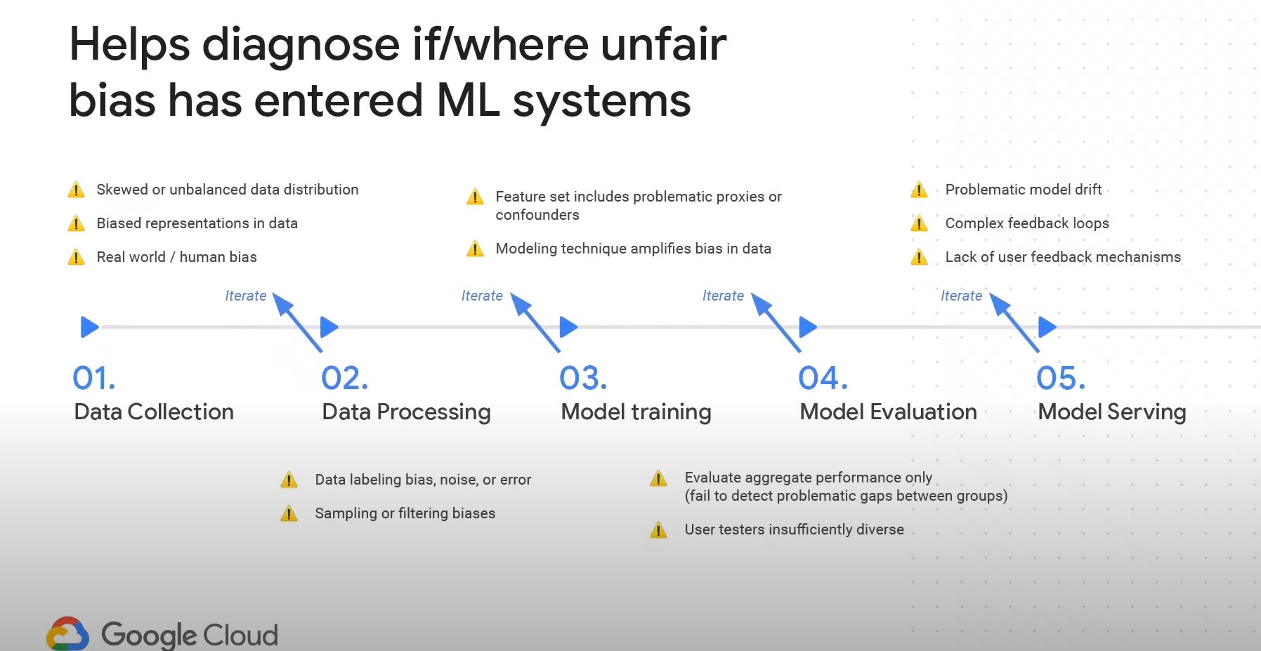
Where can bias occur in ML? Everywhere

• Modeling technique can amplify bias (Example: If the loss measures mean squared error, it tends to highlight extreme values. If the loss measure is mean absolute error, it tends to ignore these extreme cases.)

• Model Evaluation can introduce bias: (Example: are we evaluating the bulk of evaluation or just a slice of it.)

• Model serving can introduce bias: (Example: Are we incorporating user feedback, is model drift happening?)

Types of interpretabliity:

• Local vs Global
• Model specific (Example: model internal visoualizaer, weight distribution in the models)
• Model agnostic
• Intrinsic interpretable models (Example: Linear Regression, Logistic Regression, LDA, K nearest neighbors, decision trees)

Scope of interpretability:

• Global holisitc interpretablity
• Explain overall model behavior Models become hard to understand in higher dimensional plane
• Explain parts of model behavior. Explain a specific prediction

Evaluation/validation of interpretation:

• No easy way
• May require human to validate
• May require domain expert to validate

Properties of explanation:

• More or less similar to how we would like any explanation:
• accurate, consistent, clear, representative, high fidelity

Exercise:

• List the common ML algorthims and techniques to interpret the model?
• List some of the common tools used for model interpretation (Examples: Lime, shap, integrated graient, xray, trick tracing)
• List some of the common questions user can ask regarding interpretation?
  • Why did the model predict a result in a specific way?
  • What are the important features for this model?
  • How do evaluate model learning?
  • How can we correct bias in the training set?

References:

• Hands on Lab: Explainable AI in GCP

Chapter 8: Global Model Agnostic Methods:

‘Having gathered these facts, Watson, I smoked several pipes over them, trying to separate those which were crucial from others which were merely incidental.’

-Sherlock Holmes in The Crooked Man

Functional Decomposition

What is Functional decomposition? It is the decompositon or break down/grouping of features to identify all possible interactions. Example: if the model is predicting the house price using three features (X = {rooms, sqft, and zip)} Then, feature compostion is:

1. intercept
2. # of rooms
3. sq ft
4. zipcode
5. # of rooms * sqft
6. # of rooms * zipcode
7. sqft * zipcode
8. # of rooms * sqft * zipcode

Thus if the features are 3, the number of components or subsets are 2^3 = 8. If features are N, then we will have 2^N components.

This is computationally expensive. Moreover, all the 2^N components are not effective or important. So how do we filter the components or prune this list?

Three methods:

• Functional ANOVA (Analysis of Variance) Hypothesis Approach:

  • First step is to test the variance between the groups are equal or similar
  • If the variance between the group divided by the variance within the group is very high, then the variable of interest is playing a higher role on the interaction.
  • Calculate variance between the groups using F-test and mean between the group by t-test
  • One way, Two ways, and K way ANOVA to evaluate different # of variables of interest.

  Model based approach:

  • The ANOVA decomposition partitions the total variance of the model, as a sum of variances of orthogonal functions for all possible subsets of the input variables.
  • This is done by integrating the values of all features except the feature of interest and variance is calculated. This process is repeated by excluding each feature (for one way variance, product of two features for two way variance and so on)
  • Total variance is calculated and compared with each of the subset variance to find if the dependent variable can be explained in low dimension without much loss.
  • Thus this process helps with feature selection by reducing high dimensionality to low dimensionality.

• Accumulated Local Effects

• Statistical regression models

  • Example linear regression (Lasso regression for feature selection)

Permutation Feature importance

• Depending on # of predictors/features, as it requires iterating through them, this can be computationally expensive
• Poor performance with multi collinearity. (Similar to the issue with Random Forest feature importance)
• Feature importance does not help with inference
  • This helps to identify important features but not its nature…
• Common python packages are (eli5, alibi, scikit-learn, LIME)

from sklearn.model_selection import train_test_split
from sklearn.ensemble import RandomForestRegressor
from sklearn.metrics import mean_squared_error

X = df.drop(columns = target)
y = df.target

X_train, X_test, y_train, y_test = train_test_split(X, y, test_size=0.33, random_state=42)

regr = RandomForestRegressor(max_depth=100, random_state=0)
regr.fit(X_train, y_train)

rmse_full_mod = mean_squared_error(regr.predict(X_test), y_test, squared = False)

results = []
# Iterate through each predictor
for predictor in X_test:

    # Create a copy of X_test
    X_test_copy = X_test.copy()
    X_test_copy[predictor] = X_test[predictor].sample(frac=1).values
    new_rmse = mean_squared_error(regr.predict(X_test_copy), y_test,
				  squared = False)

    # Append the increase in MSE to the list of results
    results.append({'pred': predictor,
		    'score': new_rmse - rmse_full_mod })
# Convert to a pandas dataframe and rank the predictors by score
resultsdf = pd.DataFrame(results).sort_values(by = 'score',
					      ascending = False)

Global Surrogate Model

#Blackbox model
 model  = RandomForestRegressor()
 model.fit(X_train, Y_train)

#Create Surrogate Model
new_target = model.predict(X_train)
surrogate_model = DecisionTreeRegressor(max_depth=10)
surrogate_model.fit(X_train, new_target)

feature_importance['importance] = surrogate_model_feature_importances_

Summary:

• All models fail if the data has correlation(PDP, Permuation feature importance, H statistic, ANOVA)

• Partial Dependence Plot summarizes the effect of a particular explanatory variable on the target variable. This is done by averaging all of the CP plots (Ceteris Paribus)

• All of the techniques mentioned here require extensive computation as the interaction has to be calculated at all subsets level which can be maximum of 2^N (for N number of independent variables/features)

• One of the recommended ways of using these techniques is to fit the model and go through a dashboard based approach of evaluating features for their correlation and interaction and then build models with low dimensional features

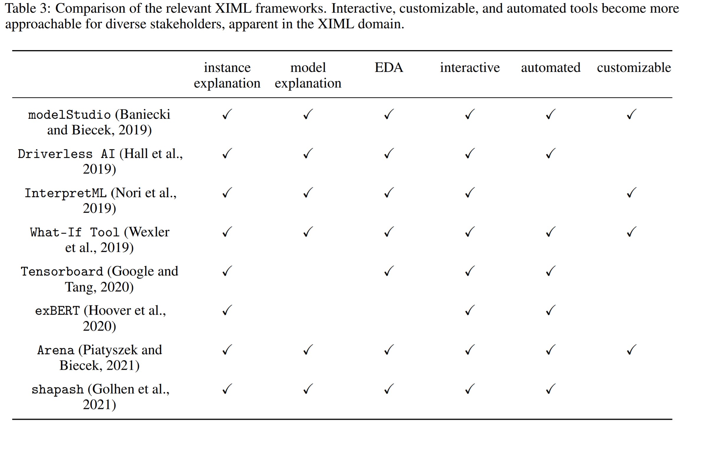
• There are many model frameworks available that can help to plot both these global and local interactions and plots. The below chart summarizes main options currently available.

References:

• Explanatory Model Analysis
• Model Studio Demo

Chapter 10: Neural Network Interpretation

Terms and Definitions:

Term	Definition
Batch normalization	Standardizing inputs for each mini batch of training set 1
Feature Attribution Methods	Algorithms to identify how much each feature is contributing to the model prediction
Channel	The depth of the matrices involved in convolutions 3
CNN	Inspired from visual cortex design in humans. Neurons respond to stimuli only in some regions called receptive field. A group of such fields overlap to cover entire visual area. Similarly in CNN, multiple channels respond to specific activation and learn parts of the overall image
Disentangled Features	Breaking down each feature to encode them as separate dimensions
Batch Propagation	Repeatedly adjusting the weights of the neurons/connections to minimize the difference between actual and output vectors.

Approaches:

Advantages	Disadvantages
Feature Visualization and network dissection provide insight into neural network	Many Images are not interpretable
Helps to communicate pixel importance in non-technical way	Provides illusion of interpretability
Helps to detect concepts in neural network layers	Data has to be labelled at pixel level
	Too many units and layers to look at in a neural network

Feature Visualization:

• Visualize learned features by activation maximization
• Identify the input(s) that maximize(s) the neuron or the layer and use this input to learn the features of the image.
• Randomly create the input or search through the training data and find an image that meets this criteria
• Hence this is an optimization problem
• Extremely time consuming.
• Activation maps is one alternative to speed this up.

Pixel activation/sensitivty maps:

• Identify the relevant and important pixels for the specific image classification
• Two methods: Each method assigns value to each pixel which can be used to interpret its relevance in the image classification
  • Occlusion or pertrubation method - Modify image pixels to generate explanations.
  • Gradient based methods - Calculate the gradient or slope of the prediction against its input features. It basically measures if change in the pixel results in improved predictions.
    • Example: Increase the color and check if the prediction results in the right probability class
• CNN is axis dependent. Random combinations of channels are less likely to detect unique concepts
• Interpretability is independent of discriminative power i.e The ability to differentiate objects remain the same, but interpretablity increases when the images are orthogonaly transformed.

Network Dissection:

• Disentangled features help in recognizing real world concepts
• Different channels learn different objects instead of all channels learning some part of the same object.
• Disentangled features mean highly interpretable. Study each channel to understand how it differentiates one object from antoher by monitoring which layers are getting activated.
• Get human assisted labelled images. The label should be at pixel level and not at image level. Run into thru CNN to see which channels are getting activated for this image.
• Lower concepts are learned at lower layers (color, textures etc) parts and objects which are higher concepts are learned at higher layers

Testing with concept activation vectors

• For a given concept, this algorithm quantifies how much the concept is influencing the prediction

• Generate two datasets..one with the concept and one without the concept.

• Train a classifier and identify the layer where there are activations for the concept images.

• The coefficient of this vector is the unit concept activation vector

• During prediction, compare how much the predicted image direction relates to the unit concept activation vector

Adversarial Examples:

• Idea is to trick the model…not interpretability
• Helps in adding rigor to the model from cyber/vulnerability attacks
  • Example: A model is developed to look for dangerous weapons. An adversarial example would be to develop a knife that looks like umbrella and passes through the security check
• These methods are developed by altering single or group of pixels in the training data to trick the model.

Influential Instances:

• Identify the instances that re influential to model prediction. i.e. if these instances are removed, then model performance significantly goes down.
• Broadly two methods:
  • Deletion Diagnostics
  • Influence Functions

Deletion Diagnostics

• Cook's Distance measures the effect of deleting influential instances from the training dataset
• Idea is to retrain the model multiple times by repeteadly removing instances and measuring the estimates and comparing them to estimates from model with all instances

Influence Functions

• In this method, influential instances are identified without multiple retraining of data by repeated inclusions/exclusions.
• Retraining is not necessary. However, this approach works only on those ML algorithms where loss gradients are accessible. So tree based models do not support this.