KubeFlow Bootcamp

Introduction to machine learning in Production (DeepLearning.AI)

Key Concepts:

• What makes deployments hard?
  • A statistical issues
  • Software Engine Issues.

Concept Drift and Data Drift:

Speech Recognition Example Pipeline: Audo is connected to VAD (Voice Activity Detection) looks at long stream of audio and clips only the part that has speech and forwards it to speech recognition module in cloud which in turn generates transcript.

Deploying Machine Learning Models in Production

Week 1 [Model Serving: Introduction]

Introduction to Model Serving

Introduction to Model Serving Infrastructure

TensorFlow Serving

Week 2 [Model Serving: Patterns and Infrastructure]

Learning Objectives

• Serve models and deliver inference results by building scalable and reliable infrastructure.
• Contrast the use case for batch and realtime inference and how to optimize performance and hardware usage in each case
• Implement techniques to run inference on both edge devices and applications running in a web browser
• Outline and structure your data preprocessing pipeline to match your inference requirements
• Distinguish the performance and resource requirements for static and stream based batch inference

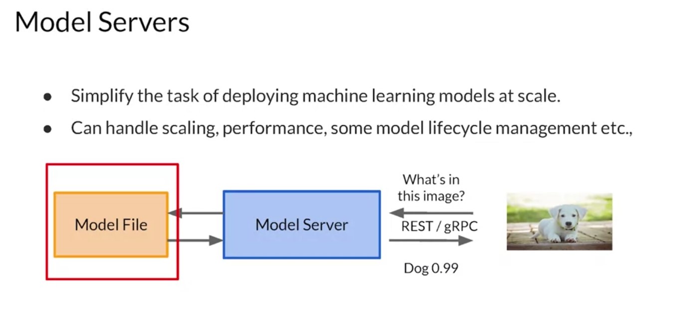
Model Serving Architecture Details

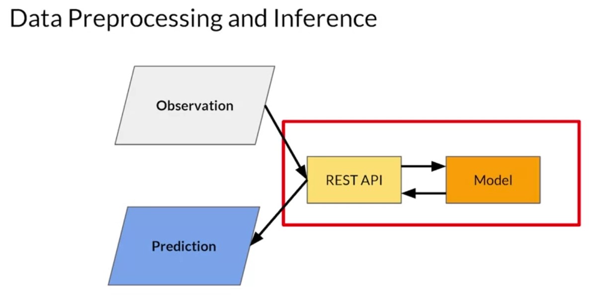
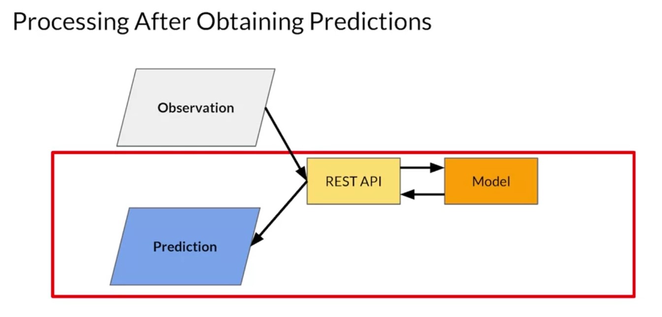
The high level architecture of a model server can be summarized in a diagram like this one. Your model is typically saved to the file system. You could also have multiple versions of the same model, so you can try out different ones. But ultimately, it’s available to be read by the model server whose job it is to instill instantiate the model and expose the methods on the model that you want to make available to your clients. So for example, if the model is an image classifier, the model itself will take in tensors of a particular size and shape. For mobile net, these would be 224 by 224 by 3. The model server receives this data formats it into the required shape, passes it to the model file and gets the inference back. It can also manage multiple model versions should you want to do things like AB testing or have different users with different versions of the model. And the model server then exposes that API to the clients as we previously mentioned. So in this case for example, it has a REST or RPC interface that allows an image to be passed to the model. The model server will handle that and get the inference back from the model, which in this case is an image classification and it will return that to the collar.

• Tensorflow Serving

  TF Serving Architecture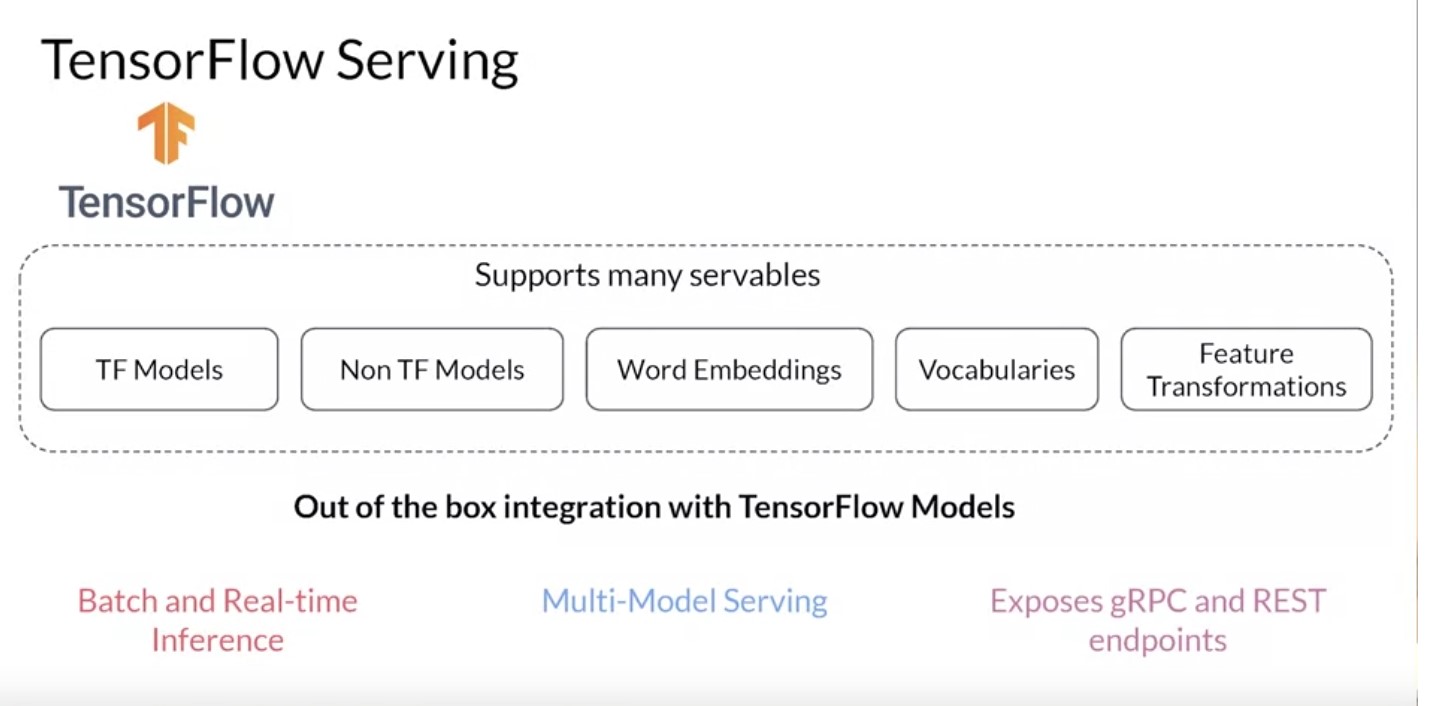

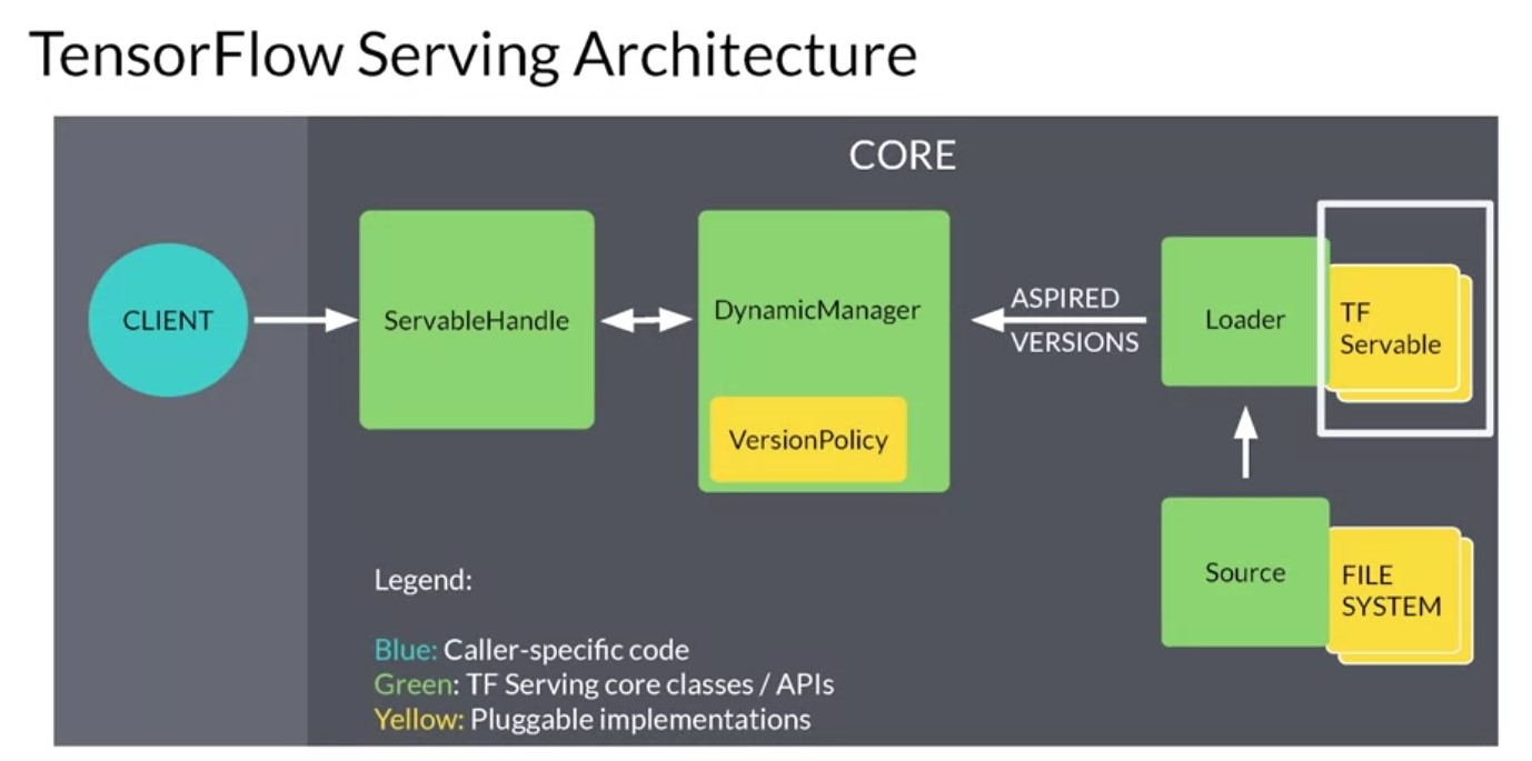
  So now that you’ve seen model serving from a high level, let’s dig into some of the architecture is a little more deeply, starting with TensorFlow Serving. In week 1, you had a chance to experiment with the basics of TF serving, which is a flexible, high performance serving system for machine learning models. It provides out of the box integration with tensorflow models and it can also be extended to serve other types of model. So let’s take a look at the architecture of this serving system and some important features that I’d like to call out our that it provides both batch and real time inference. So you can either get a bunch of inferences at the same time, which is useful if you’re building something like a recommendation engine. That requires a lot of predictions or real time inference if you want to answer to a single task back quickly. And this is useful for for example, an image classification. Multi model serving is also available and this allows you to have multiple models for the same task and the server chooses between them. This could be useful for example, for a b testing audience segmentation and more. And it also provides remote procedure calls or traditional rest endpoints on which you can call your server. The high level architecture for tensorflow serving looks like this. It’s built around the core idea of a servable, which is the central abstraction in TF serving. These are the underlying objects that clients used to perform computation. For example, inference or lookups. There can be any kind of type or interface and this makes them very flexible. A typical servable is a tensorflow saved model but it could also be something like a look up table for an embedding. The loader manages a survivals lifecycle. The loader API enables common infrastructure independent from specific learning algorithms, data or whatever product use cases were involved. Specifically loaders standardized the API is for loading and unloading a servable. Together these produce aspired versions and these represent the set of servable versions that should be loaded and ready. Sources communicate this set of servable versions for a single servable stream at a time when a source gives a new list of aspired versions to the manager. It supersedes the previous list for that servable stream. The manager unloads any previously loaded versions that no longer appear in the list. The Manager then handles the full life cycle of the survivals, including loading the survivals serving the survivals and of course unloading the survivals. The managers will listen to the sources and will track all of the versions according to a version policy and the servable handle provides the exterior interface to the client. There’s a lot of pieces here. So let’s look at an example of how this would work. So let’s take this as an example, say a source represents a tensorflow graph with frequently updated model weights. The weights are stored in a file and disk. The source detects a new version of the model weights. It creates a loader that contains a pointer to the model data on disk. The source notifies the dynamic manager of the aspired version. The dynamic manager applies the version policy and decides to load the new version. The dynamic manager tells the loader that is enough memory. The loader instantiates the tensorflow graph as a servable with these new weights. A client requests a handle to the latest version of the model and the dynamic manager returns a handle to the new version of the servable. You can then run inference using that servable and this is what you would have seen last week when you built the fashion MNIST model example.

• Nvidia Triton Server

  TF Serving Architecture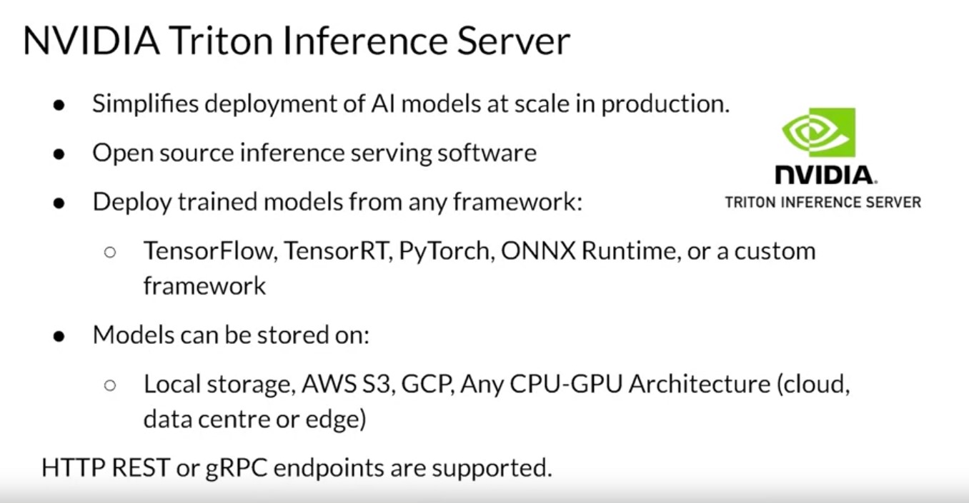

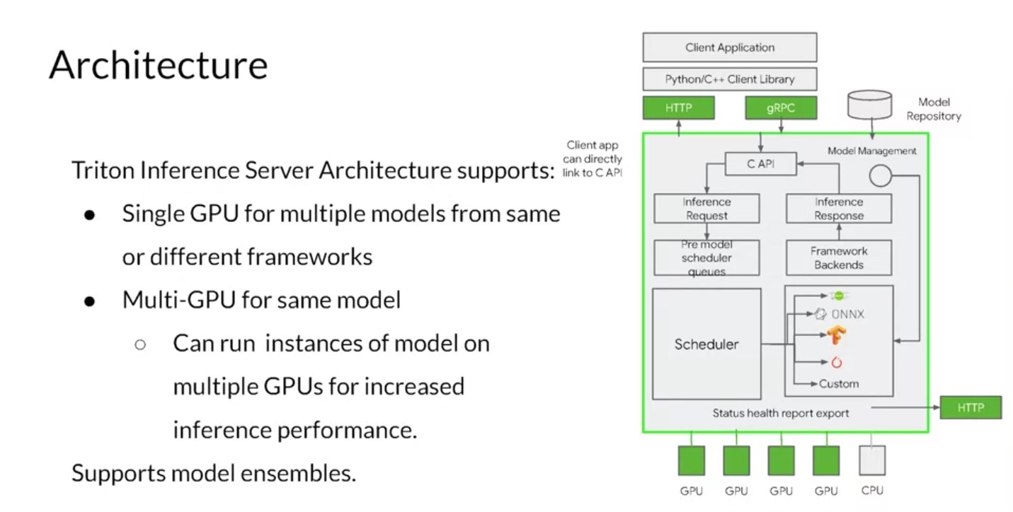
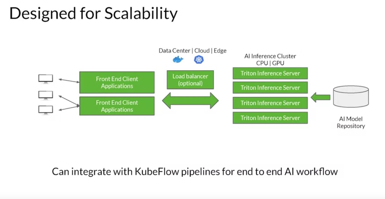
  The Triton Inference Server, an offering from NVIDIA, simplifies deployment of AI models at scale in production. It’s an open-source inference serving software that lets teams deploy trained AI models from any framework: TensorFlow, TensorRT, PyTorch, ONNX Runtime, or even a custom framework. You can deploy from local storage or from a Cloud platform, like the Google Cloud Platform or AWS, on any GPU or CPU-based infrastructure. It can be the Cloud, the data center, or even the edge. The Triton Inference Server runs multiple models from the same or different frameworks concurrently on a single GPU using CUDA streams. In a multi-GPU server, it automatically creates an instance of each model on each GPU. All of these increase your GPU utilization without any extra coding from the user. The Inference server supports low latency real-time inferencing with batch inferencing to maximize GPU and CPU utilization. It also has built-in support for streaming inputs if you want to do streaming inference. Users can use shared memory support for higher performance. Inputs and outputs need to be passed to and from Triton’s Inference Server can be stored in the systems or the CUDA shared memory. This can reduce the HTTP C or gRPC overhead and increase overall performance. It also supports model ensemble. Triton Inference Server integrates with Kubernetes for orchestration, metrics, and auto scaling. Triton also integrates with Kubeflow and Kubeflow Pipelines for an end-to-end AI workflow. The Triton Inference Server exports Prometheus metrics for monitoring GPU utilization, latency, memory usage, and inference throughput. It supports the standard HTTP gRPC interface to connect with other applications like load balancers. It can easily scale to any number of servers to handle increasing inference loads for any model. The Triton Inference Server can serve tens or hundreds of models through the Model Control API. Models can be explicitly loaded and unloaded into and out of the Inference server based on changes made in the model control configuration to fit in a GPU or CPU memory. It can be used to serve models and CPU too. It supports heterogeneous cluster with both GPUs and CPUs and does help standardized inference across these platforms. During peak loads, it can dynamically scale out to any CPU or GPU.

• Torch Server

  Torch Serving Architecture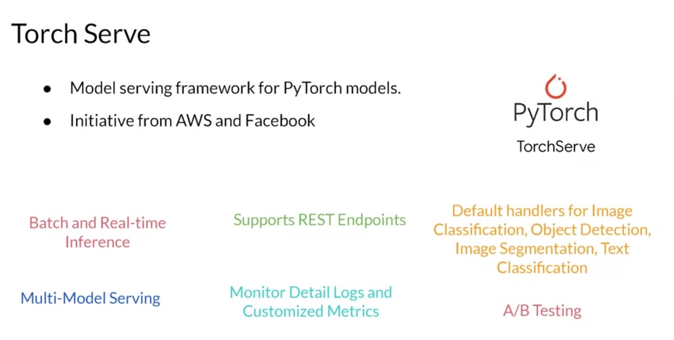

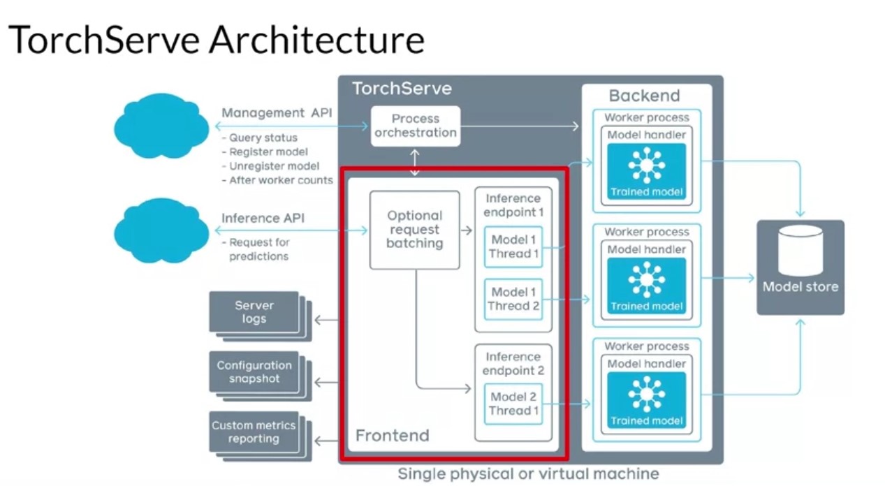
  TorchServe is an initiative by AWS and Facebook to build a model serving framework for PyTorch models. Before the release of TorchServe, if you wanted to serve PyTorch models, you had to develop your own model serving solutions like custom handlers for your model, you had to develop a model server, maybe build your own Docker container. You had to figure out a way to make the model accessible via the network and integrated it with your cluster orchestration system and all of that good stuff. With TorchServe, you can deploy PyTorch models in either eager or graph mode. You can serve multiple models simultaneously. You can have version production models for A/B testing. You can load and unload models dynamically and you can monitor detail blogs and customizable metrics. Best of all, TorchServe is open source. Hence it’s extensible to fit your deployment needs. The server architecture looks like this. The front end is responsible for handling your requests and your responses. It handles both requests and responses coming in from clients and the model life cycle. The back end users model workers that are running instances of the model loaded from a model store. They’re responsible for performing the actual inference. You can see that multiple workers can be run simultaneously on TorchServe. They can be different instances of the same model or they could be instances of different models. Instantiating more instances of a model enables handling more requests at the same time and can increase the throughput. A model is loaded from cloud storage or from local hosts. TorchServe support serving of eager mode models and jet saved models from PyTorch. The server supports APIs for management and inference, as well as plugins for common things like server logs, snapshots, and reporting.

• KubeFlow Serving

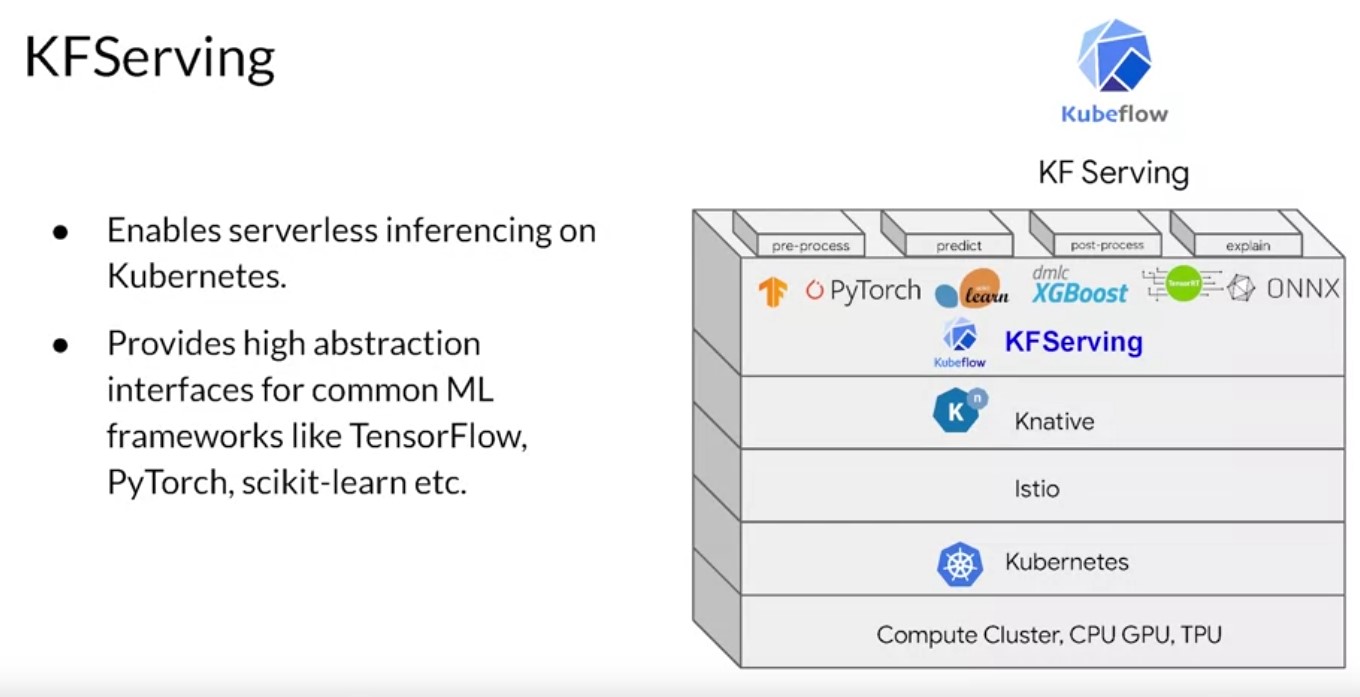  Kubeflow Serving. There’s a bit too much to go into detail here, but let’s look at it briefly. Kubeflow also offers serving capabilities with Kubeflow Serving. This allows you to use a compute cluster with Kubernetes to have serverless inference through abstraction. It works with TensorFlow, PyTorch and others. I won’t go into the detail on it here, but you can learn more about it at the URL provided in the additional readings. Now that you’ve seen how serving of machine learning models can be achieved, let’s take a step back and explore scaling applications like these. You can understand the fundamentals of horizontal and vertical scaling. From there, you’ll see how you can use virtualization, containers, and container orchestration to manage the serving of your apps at an appropriate scale using open-source services.

Scaling Infrastructure

Online Serving

Data PreProcessing

Data Preprocessing		Post Process

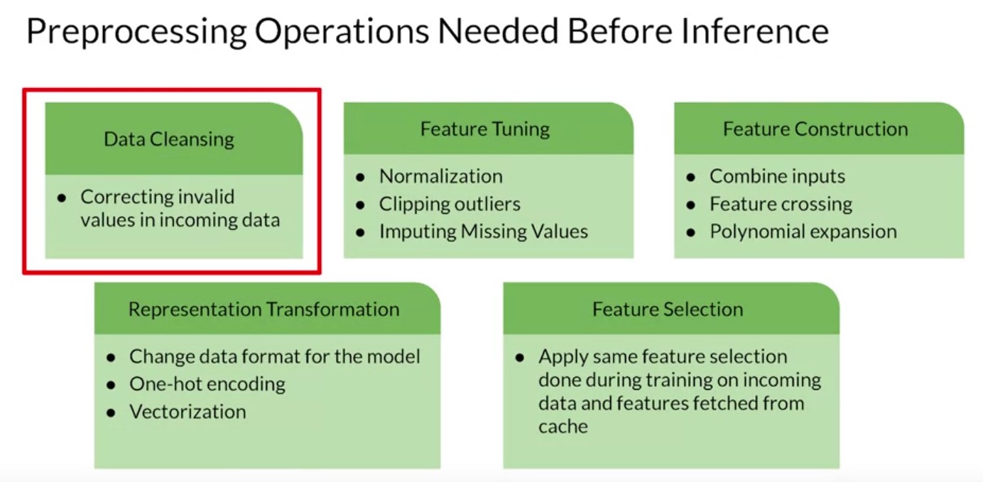
So let’s start to look and start by considering the input data to your app. If you go back to this very simple high level diagram of an app, remember that the observation data being passed into the system may be in one format but that’s not necessarily the same format that the model was designed to take in. The data has to be converted somehow. So, for example, consider a simple language model where maybe the observation is a sentence that the user typed and is stored as a strength. The model is designed to classify that text to see if it’s toxic. NLP models like this are trained on input vectors where words are transformed into a high dimensional vector and sentences are sequences of these vectors. Now that pre processing of the data has to be done somewhere. And that’s just a relatively simple example of where you need to do a translation of data from one format to another. Other areas to consider when pre processing are things like data cleansing where you correct invalid values in incoming data. For example, maybe you’re building an image classifier and the user sends you a picture that’s invalid because it’s too big. You could reject it, of course, or you could take on the process of re-sizing it to get a valid picture size. Then there’s feature tuning where you do some transformation on the data to make it suitable for the model. In the case of an image, this could be normalization where instead of us having a 32 bit value to represent a pixel, you might convert it to three 8 bit values for red, green and blue, ignoring the alpha channel. And then instead of these having values between 0 and 255, you could convert them to values between 0 and 1 as neural networks tend to deal better with normalized values like that. Or with the example of a string coming in, its encoding the string into the vocabulary representation that the model uses, which could clip outliers such as infrequently used words. Often models will require data pre processing to involve feature construction. So for example, when it comes to a model that, for example, might predict the price of a house, the input data might have multiple columns such as the number of rooms and the size of each, but the model is trained on the total floor space of the house. So then feature crossing could be used to multiply the values that you have out to get the feature type that the model uses. Other scenarios here could be a polynomial expansion where a new feature is calculated from a formula of the original feature. Maybe the data contains temperature in Celsius but the model expects Fahrenheit.

Batch Inferencing Scenarios

• Overview

  

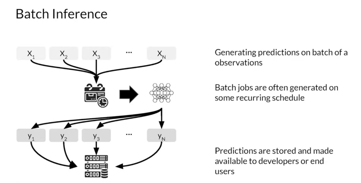
  You’ve looked at model scaling as well as architectures for inference. Now let’s consider model performance and resource requirements for batch inference. After you train, evaluate and tune a Machine Learning model. The model is deployed to production to generate predictions. An ML model can provide predictions in batches which will be applied to a use case at sometime in the future. Prediction based on batch inference is when your ML model is used in a batch scoring job for a large number of data points where predictions are not required or not feasible to generate in real-time.

  • In batch recommendations, for example, you might only use historical information about customer item interactions to make the prediction without any need for real-time information.
  • Batch recommendations are usually performed in retention campaigns for inactive customers that have a high propensity to churn or in promotion campaigns and stuff like that. Batch jobs for prediction are usually generated on some recurring schedule like daily, at night or maybe weekly. Predictions are usually stored in a database that can then be made available to developers or end-users.

  Advantages

  

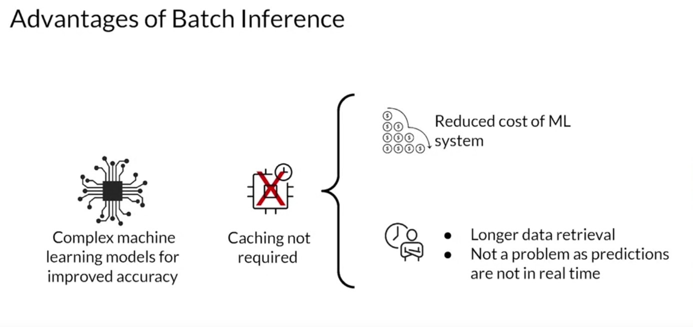
  • Complex machine learning models can be used to improve the accuracy of predictions since there’s no constraint on inference time.
  • Caching of predictions is usually not required.
  • Employing a caching strategy for features needed for prediction is also not required.
  • Batch inference can wait for data retrieval to make predictions since the predictions are not available in real-time.

  Disadvantages

  

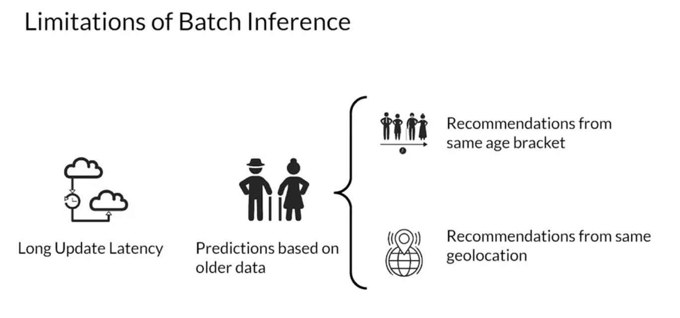
  • Predictions cannot be made available for real-time purposes.
  • Latency in updating predictions can be hours or sometimes even days.
  • Predictions are often made using old data. This is problematic in certain scenarios.
    • Suppose a service like a movie streaming generates recommendations at night. If a new user signs up they may not be able to see personalized recommendations right away.
    • Usual workaround is the system shows recommendations from other users in a similar demographic like the same age bracket or maybe the same geolocation as a new user.

  Important Metric

  • The important metric to optimize while performing batch predictions is throughput.
  • Always increase throughput in batch predictions rather than the latency.
  • The model should be able to process large volumes of data at a time.
  • As throughput increases the latency with which each prediction is generated increases also. But this is not a big concern in batch prediction systems since predictions need not be available immediately.
  • Predictions are usually stored for later use and hence, latency can be compromised.
  • Throughput of an ML model or Production System processing data in batches can be increased by usage of hardware accelerators like GPUs, TPUs.
  • Increasing the number of servers or workers in which the model is deployed is another option.
  • Anotherw way is to load several instances of the models and multiple workers to increase the throughput.

  Use Cases

  Use Case - Recommendation System	Use Case: Sentiment Analysis	Use Case: Time Series Forecasting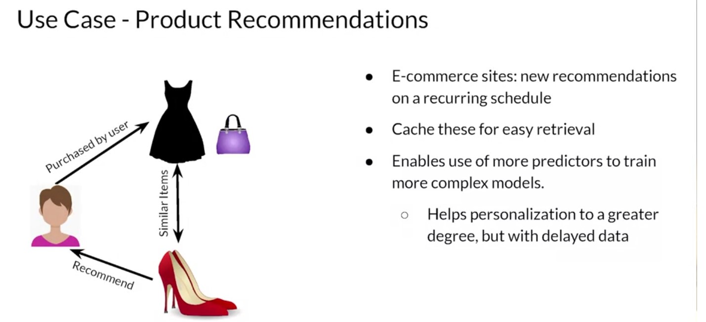

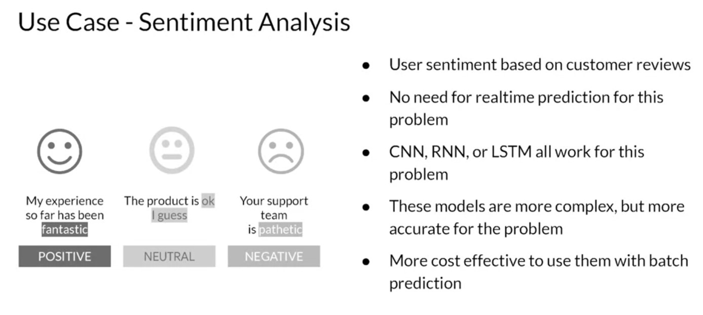
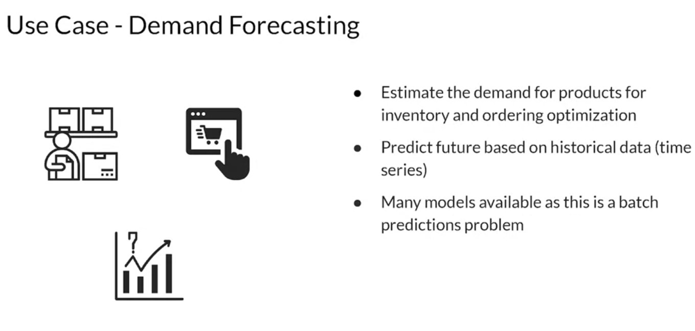
  First, new product recommendations on an e-commerce site can be generated on a recurring schedule. Then caching these predictions for easy retrieval rather than generating them every time you use a logs in makes it much easier. This can save inference costs since you don’t need to guarantee the same latency as real-time inference needs to have. You can also use more predictions to train more complex models since you don’t have the constraint of prediction latency. This helps personalization to a greater degree but using delayed data that may not include new information about the user. Let’s look at a sentiment analysis problem. Based on the users reviews, usually in text format, you might want to predict if a review was positive, neutral or negative. Systems that analyze user sentiment for your products or services based on customer reviews can make use of a batch prediction on a recurring schedule. Some systems might generate products sentiments on a weekly basis, for example. Real-time prediction is not needed in this case since the customers and stakeholders are not waiting to complete an action in real time based on the predictions. Sentiment predictions can be used for improvements of services or products over time. As you can see, it’s not really a real-time business process. A CNN, RNN or LSTM based approach can be used for sentiment analysis. I tend to like LSTM. These models are more complex but they often provide higher accuracy. That makes it more cost-effective for you to use them with batch prediction. Let’s look at a different example, forecasting demand for products or services. You can use batch predictions for models that estimate the demand for your products perhaps on a daily basis for inventory and ordering optimization. It can be modeled as a time series problem since you’re predicting future demand based on historical data. Since batch predictions have minimal latency constraints, time series models like AROMA, SARIMA or an RNN can be used over approaches like linear regression for more accurate prediction.

Batch Processing with ETL

Week 3 [Model Management and Delivery]

ML Experiments Management and Workflow Automation

MLOPs Methodology

Model Management and Deployment Infrastructure

Week 4 [Model Monitoring and Logging]

Model Monitoring and Logging

Model Decay

GDPR and Privacy

---

MLOPs fundamentals from Google Cloud (Coursera)

Some of the things we hear from data scientists are:

• keeping track of the many models we have trained is difficult.
• They want to keep track of the different versions of the code,
• the values they chose for the different hyperparameters, and
• the metrics they’re evaluating. They have trouble keeping track of which ideas had been tried,
• which ones worked, and which ones did not.
• They cannot pinpoint the best model, which is possibly trained two weeks previously, reproduce it, and run it on full production data.
• Reproducibility is a major concern because there are scientists who want to be able to re-run the best model with a more thorough parameter sweep.
• Putting a model in production is difficult unless it can be reproduced, because many companies have that as a policy or requirement.

Introduction to Kubernetes and containers:

Containers are isolated user spaces for running application code. Containers are lightweight because they don’t carry a full operating system, they can be scheduled or packed tightly onto the underlying system, which is very efficient. They can be created and shut down very quickly because you’re just starting and stopping the processes that make up the application and not booting up an entire VM and initializing an operating system for each application.

The container allows you to execute your final code on VMs without worrying about software dependencies like application run times, system tools, system libraries, and other settings. You package your code with all the dependencies it needs, and the engine that executes your container, is responsible for making them available at runtime.

containers make it easier to build applications that use the microservices design pattern. That is, loosely coupled, fine-grained components. This modular design pattern allows the operating system to scale and also upgrade components of an application without affecting the application as a whole.

• References